Finding the track lanes, Part IV

As a quick recap from last time, we started with this image: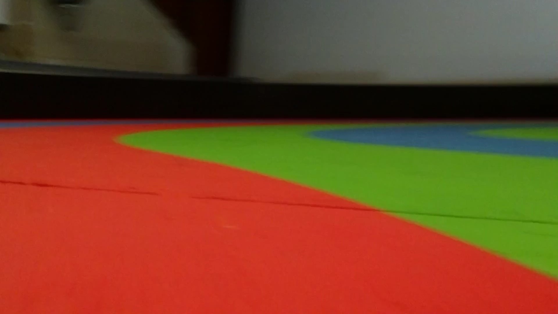
and using some processing we got to this: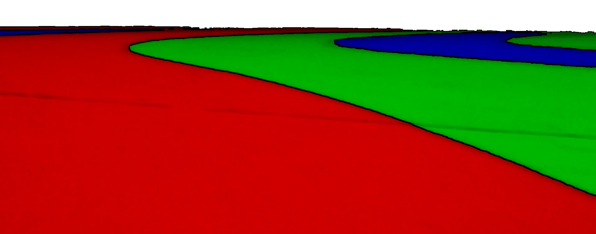
then we did some further processing to arrive at some points: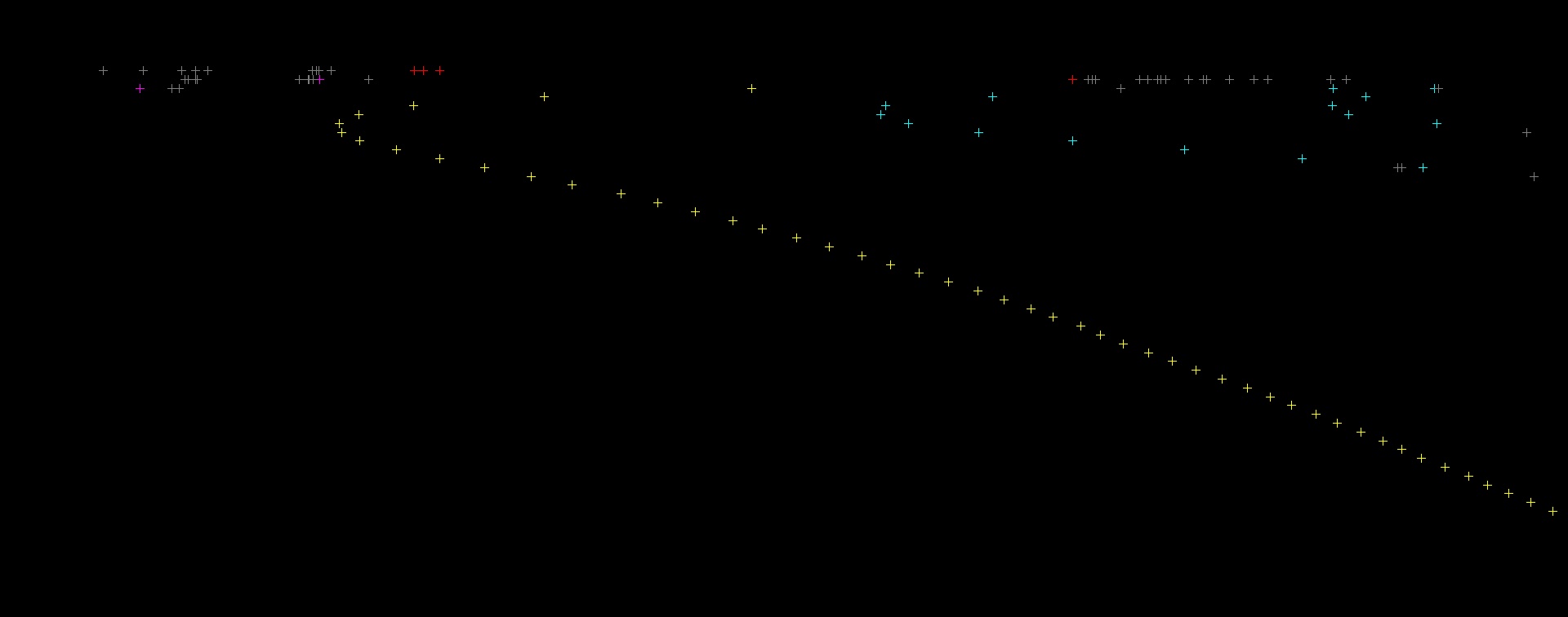
We then picked the best line to work from based on the number of points available.
Finally we calculated that the YetiBorg is at an offset of -0.124, about 12% of a lane to the right of the center.
We will be continuing the code from the previous part, which you can find here:
Finding the track lanes, Part III
In the previous part we concluded that the matchRG line was the best one to work from.
This was stored in bestLine and in our example contains 49 points.
What we want to do now is try and judge where the track is heading next.
The first thing is to measure what angle it is at:
This will be the value returned from the CurrentAngle() Race Code Function.
We can measure this by comparing how far apart each point is in X verses Y compared to the one before it.
These changes in the numbers we will refer to as dX and dY: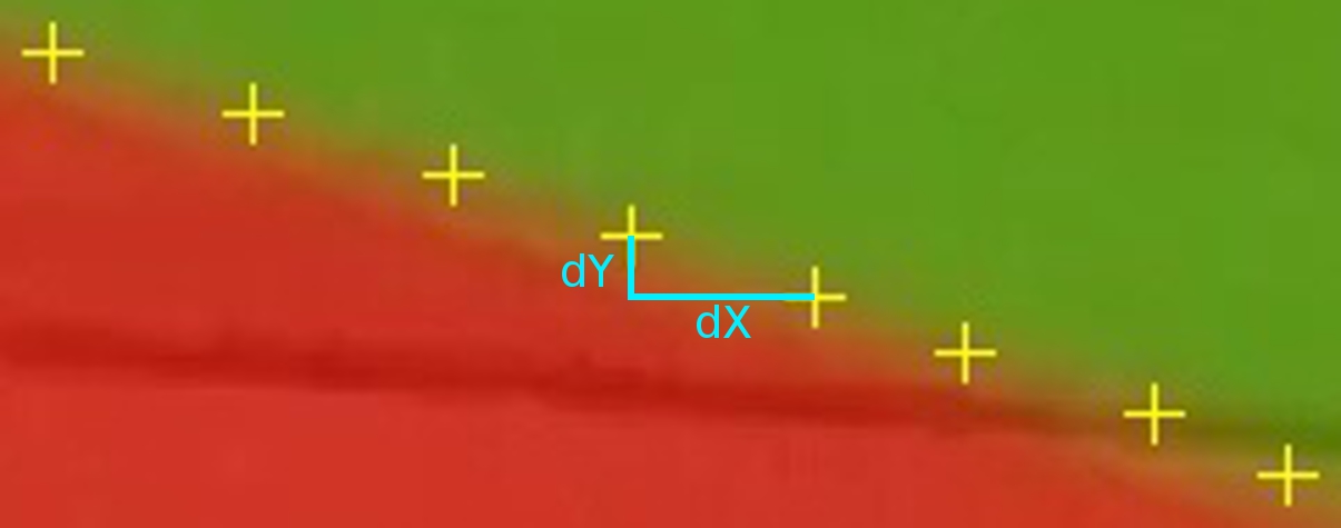
We can calculate a list of these values like so:
dXdY = []
for i in range(1, len(bestLine)):
	dX = float(bestLine[i-1][0] - bestLine[i][0])
	dY = float(bestLine[i][1] - bestLine[i-1][1])
	dXdY.append((dX, dY))
We use float to allow these values to have a fractional value later on.
To work out the amount the angle the line is at we need to divide dX by dY.
For example if X is always the same (dX = 0) and Y changes by 10 each time (dY = 10) then dX ÷ dY = 0, in other words 0°.
If X and Y both change by 10 each time (dX = 10, dY = 10) then dX ÷ dY = 1, in other words 45°.
To get an average change we simply average these values:
gradient = 0
for changes in dXdY:
	gradient += changes[0] / changes[1]
gradient /= len(dXdY)
This give use about -1.862, which is way too much (about 60°).
So why is it too much?
Consider this image: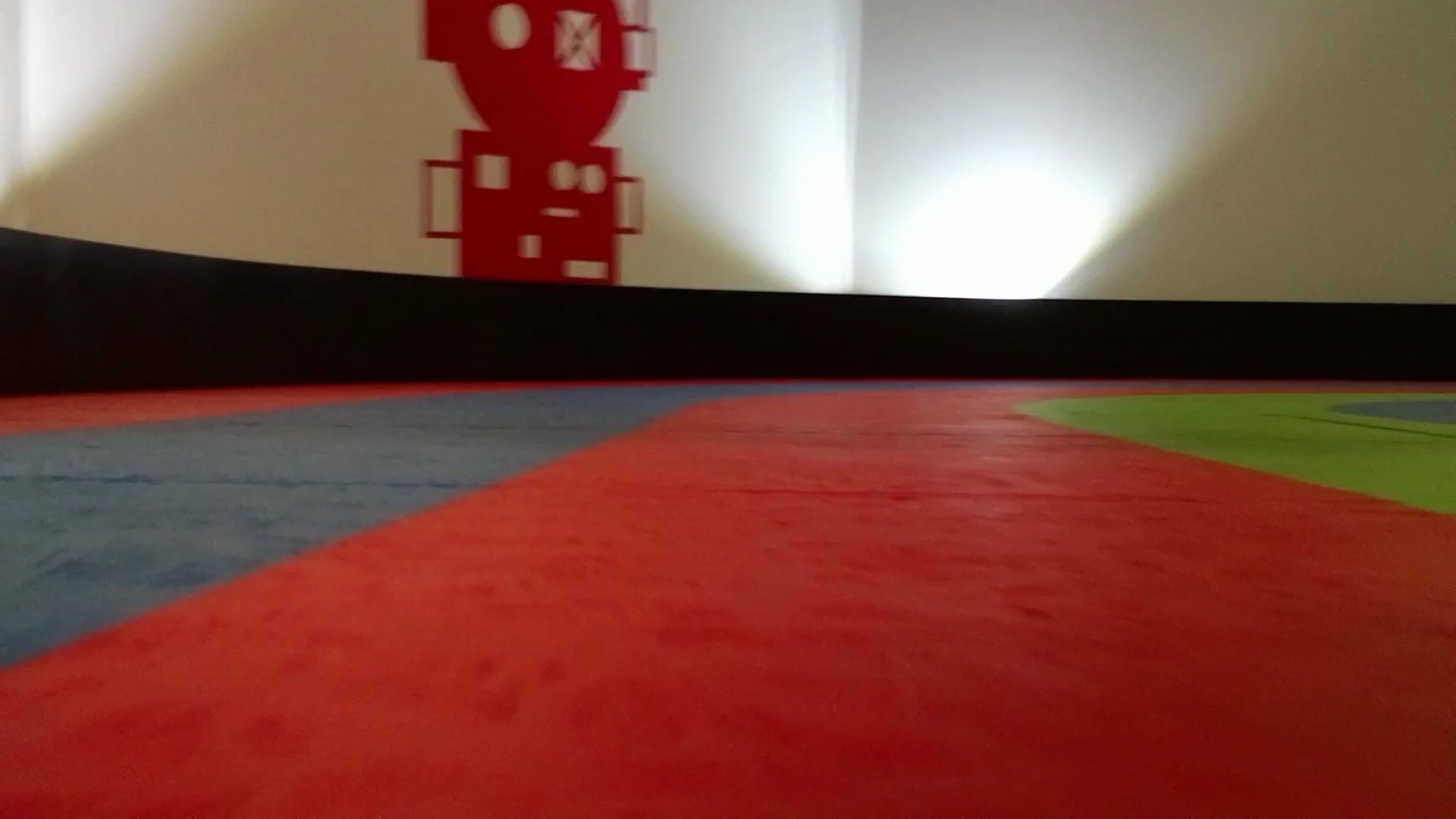
The YetiBorg is basically central (around 0°), but the lines in the image are angled.
Also notice how the angle for the lines further from the center of the image are worse?
This is called perspective error.
In order to correct for this error we need to measure the error in a 0° image.
In this case we see a gradient of about 2.6 at an offset of about 0.25 of a lane.
The offset matters as the error will scale with this offset.
Note the offset between the center of the image and the line, the value in offsetX from last time.
We can work out our correction factor as:
correctionFactor = 2.6 / 0.25
based on our measured values, about 10.4 in this case.
What this means is that we expect the gradient to be about 10.4 when we are a whole lane away from the line but facing 0°.
Note that this value is dependant on the image resolution, changing it will require the correction factor to be measured again.
We can now work out the corrected gradient for our offset like this:
correction = correctionFactor * offsetX
gradient -= correction
This gives about -0.572, much closer to the truth :)
This gradient value is what our code feeds into the later calculations.
You can get the angle returned by CurrentAngle() with a quick conversion:
angle = math.atan(gradient) * 180 / math.pi
This gives about -30 degrees, which sounds about right: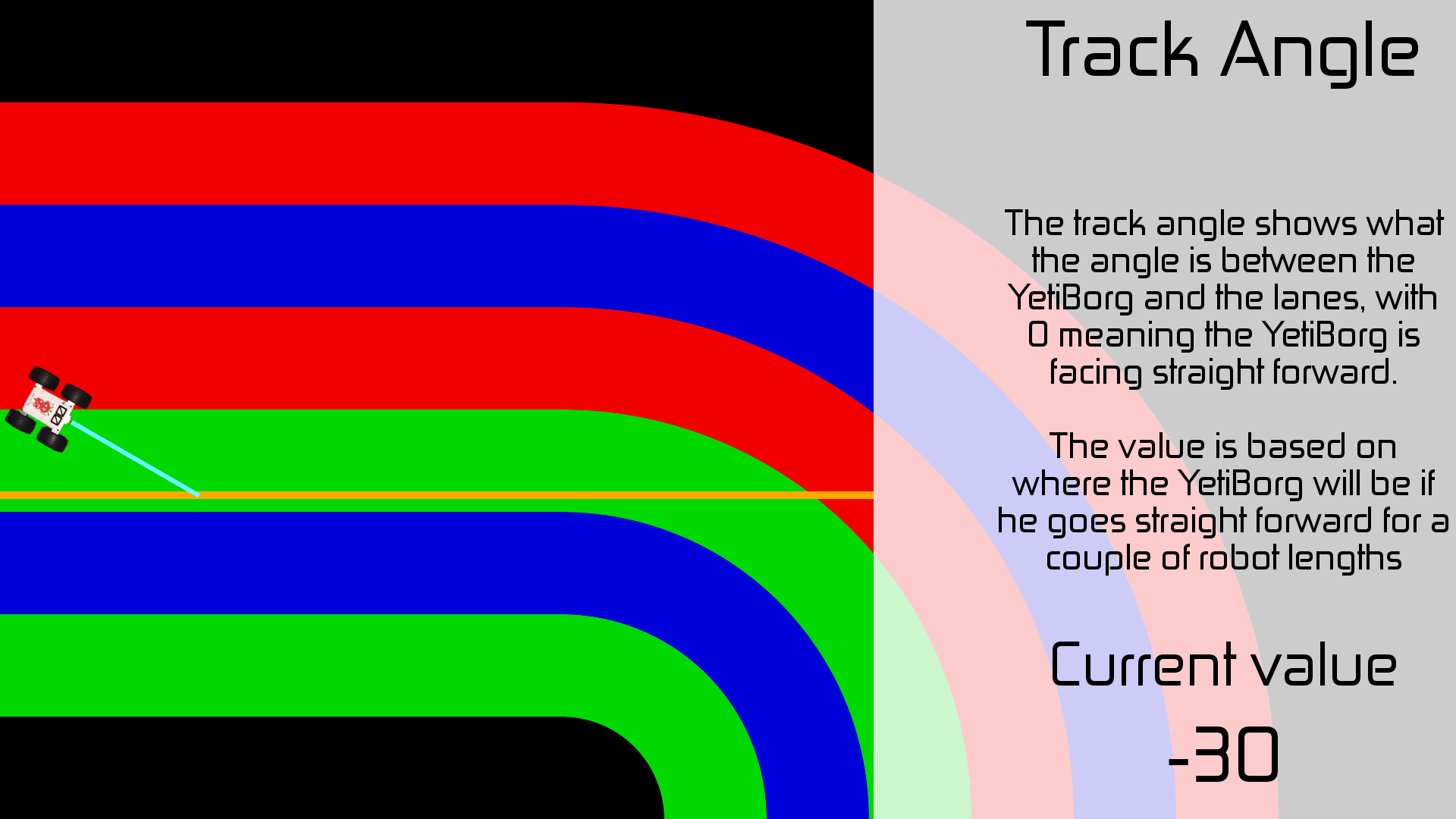
At this point you might be wondering why we stored all of the dX and dY values.
We still need these to calculate our track curvature value:
This will be the value returned from the TrackCurve() Race Code Function.
We can measure this by comparing how different the changes between points are.
Consider two measured changes when on a curve: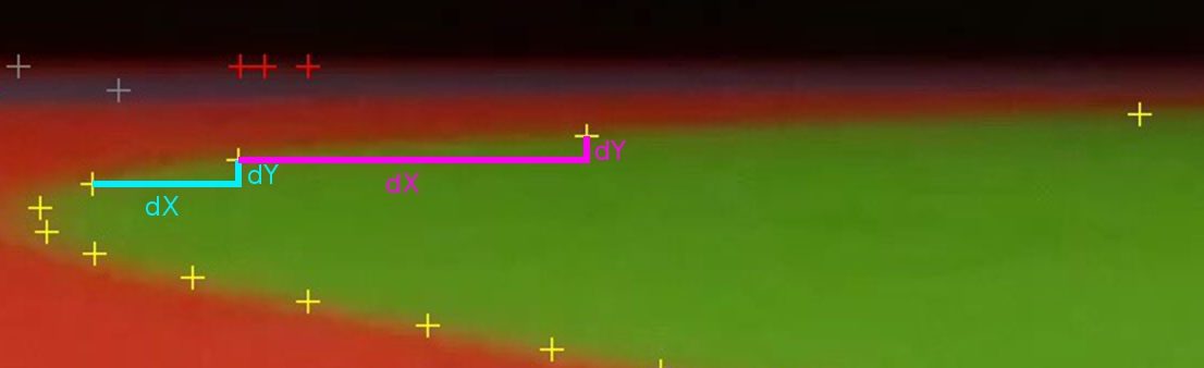
The second change is about the same for Y, but much larger in X.
This means the changes are growing as the curve bends, large growth means a sharper curve.
When looking at these changes:
- A perfectly straight line will give 0
- A gentle curve to the left sees negative changes
- A sharp curve to the left sees large negative changes
- A gentle curve to the right sees positive changes
- A sharp curve to the right sees large positive changes
We calculate this in a similar way as the first set of changes, but using the dXdY values this time:
gradient2 = 0.0
lastG = dXdY[0][0] / dXdY[0][1]
for i in range(1, len(dXdY)):
	nextG = dXdY[i][0] / dXdY[i][1]
	changeG = lastG - nextG
	gradient2 += changeG / dXdY[i][1]
	lastG = nextG
gradient2 /= len(dXdY)
This gradient2 value is the number returned from TrackCurve().
It gives a really odd reading of about 0.053 for our image.
The reason we do not get a clear "curving to the right" like we expect is because there are actually two curves: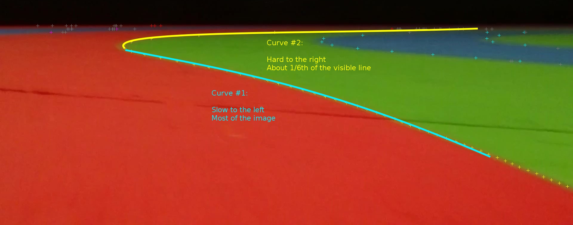
As the values get larger for both the sharpness of the curve and the number of points involved these two balance each other out.
As the robot moves forward we should see more of curve #2 and less of curve #1, giving a clearer reading of the curvature of the track.
At this point we have all of the values we should need to make decisions about where to go.
We can now pass these results on to a control loop to change the direction of the YetiBorg and start processing the next camera frame.
Add new comment